import numpy as np
import matplotlib.pyplot as plt
from mpl_toolkits.mplot3d import Axes3D  # For 3D plotting
import scipy.stats as stats

# Set random seed for reproducibility
np.random.seed(42)

# Configure plotting style
plt.style.use('ggplot')
plt.rcParams['figure.figsize'] = [10, 6]
plt.rcParams['axes.grid'] = True
plt.rcParams['font.size'] = 12Itô Process
In the previous chapter, we introduced the basic form of Brownian motion: \[ d S=\mu S d t+\sigma S d X \]
Building on this foundation, we now introduce a more general stochastic process called the “Itô process”, which can be defined as: \[ dx = a(x, t) dt + \sigma (x, t) dX \] where both the drift term \(a(x,t)\) and the diffusion term \(\sigma(x,t)\) are time-dependent functions.
To work with this process numerically, we can discretize it: \[ \Delta x=a(x, t) \Delta t+\sigma(x, t) \epsilon \sqrt{\Delta t}, \quad \epsilon \sim \mathcal{N}(0,1) \]
For any differentiable function \(G(x, t)\), we can write its Taylor expansion: \[ \Delta G=\frac{\partial G}{\partial x} \Delta x+\frac{\partial G}{\partial t} \Delta t+\frac{1}{2} \frac{\partial^2 G}{\partial x^2} \Delta x^2+\frac{\partial^2 G}{\partial x \partial t} \Delta x \Delta t+\frac{1}{2} \frac{\partial^2 G}{\partial t^2} \Delta t^2+\cdots \]
This expansion will be crucial in deriving Itô’s lemma, one of the fundamental tools in stochastic calculus.
Deriving Itô’s Lemma
Itô’s Lemma is one of the most fundamental results in stochastic calculus. It provides a way to compute the differential of a function of a stochastic process. To understand its derivation, let’s first recall some key properties of the Wiener process.
Properties of the Wiener Process
For a Wiener process \(dX\), the increments over small time intervals \(dt\) have two crucial properties: 1. \(\mathbb{E}[dX] = 0\) (zero mean) 2. \(\mathbb{E}[(dX)^2] = dt\) (variance scales with time)
These properties arise from the fact that \(dX \sim \mathcal{N}(0, dt)\), i.e., the increments follow a normal distribution with mean 0 and variance \(dt\).
The Derivation
When we consider the Taylor expansion of \(\Delta G\), most higher-order terms can be dropped as \(\Delta t \to 0\). However, the \((\Delta x)^2\) term requires special attention because: - It contains \((dX)^2\) - Due to the properties of Brownian motion, \((dX)^2 = dt\) in the limit - Therefore, this term is of the same order as \(dt\) and cannot be dropped
Substituting \(\Delta x\) and keeping only terms up to order \(dt\): \[ \Delta G = \frac{\partial G}{\partial x} (a(x, t) dt + \sigma(x, t) dX) + \frac{\partial G}{\partial t} dt + \frac{1}{2} \frac{\partial^2 G}{\partial x^2} \sigma^2(x, t) (dX)^2 \]
Using the fact that \((dX)^2 = dt\) in the limit, we obtain Itô’s Lemma: \[ dG = \left( \frac{\partial G}{\partial x} a(x, t) + \frac{\partial G}{\partial t} + \frac{1}{2} \frac{\partial^2 G}{\partial x^2} \sigma^2(x, t) \right) dt + \frac{\partial G}{\partial x} \sigma(x, t) dX \]
This formula is the stochastic calculus analog of the chain rule from ordinary calculus, but with an additional term involving the second derivative. This extra term is what makes stochastic calculus fundamentally different from ordinary calculus.
And this completes the derivation of Itô’s Lemmma.
Infinitesimal Generator
The infinitesimal generator \(\mathcal{L}\) of a stochastic process is an operator that acts on a function \(G(x, t)\) to produce another function that describes the expected rate of change of \(G\) due to the stochastic process alone, ignoring any explicit time dependence.
Given Itô’s Lemma, the infinitesimal generator \(\mathcal{L}\) can be derived by focusing on the drift and diffusion components that affect the change in \(G(x, t)\), excluding the direct time derivative term.
\[ G(x+\Delta x, t+\Delta t) \approx G(x, t)+\Delta G . \]
Taking the expectation on Ito’s lemma: Note that \(\mathbb{E}[\epsilon]=0\) and \(\mathbb{E}\left[\epsilon^2\right]=1\). Thus, the expectation of \(\Delta G\) : \[ \begin{align} \mathbb{E}[\Delta G]&=\mathbb{E}\left[\frac{\partial G}{\partial x} a(x, t) \Delta t+\underbrace{\frac{\partial G}{\partial x} \sigma(x, t) \epsilon \sqrt{\Delta t}}_{E(\cdot)=0}+\frac{\partial G}{\partial t} \Delta t+\frac{1}{2} \frac{\partial^2 G}{\partial x^2} \sigma^2(x, t) \Delta t\right] \\ \mathbb{E}[\Delta G]&=\frac{\partial G}{\partial x} a(x, t) \Delta t+\frac{\partial G}{\partial t} \Delta t+\frac{1}{2} \frac{\partial^2 G}{\partial x^2} \sigma^2(x, t) \Delta t \end{align} \]
The infinitesimal generator \(\mathcal{L}\) applied to \(G(x, t)\) is thus obtained by taking the expectation of the stochastic part of \(dG\) and is given by: \[ \mathcal{L}G = \lim_{\Delta t \to 0} \frac{\mathbb{E}[G(x + \Delta x, t + \Delta t) - G(x, t)]}{\Delta t} =\lim _{\Delta t \rightarrow 0} \frac{\mathbb{E}[\Delta G]}{\Delta t} \]
Arrange a bit: \[ \mathcal{L}G = \frac{\partial G}{\partial x} a(x, t) + \frac{1}{2} \frac{\partial^2 G}{\partial x^2} \sigma^2(x, t) \]
Chapman-Kolmogorov Equation
The Chapman-Kolmogorov Equation
Definition and Interpretation
The Chapman-Kolmogorov equation is a fundamental identity for Markov processes that describes how probability distributions evolve over time. For a Markov process \(X_t\), it states that the probability of transitioning from state \(x_0\) at time \(t_0\) to state \(x\) at time \(t+\Delta t\) can be obtained by considering all possible intermediate states \(x'\) at time \(t\):
\[ p\left(x, t+\Delta t \mid x_0, t_0\right)=\int_{-\infty}^{\infty} p(x, t+\Delta t \mid x', t) p\left(x', t \mid x_0, t_0\right) d x' \]
Key Components
- Transition Probabilities:
- \(p(x, t+\Delta t \mid x', t)\): probability of going from \(x'\) to \(x\) in time interval \([t, t+\Delta t]\)
- \(p(x', t \mid x_0, t_0)\): probability of going from \(x_0\) to \(x'\) in time interval \([t_0, t]\)
- Integration: The integral sums over all possible intermediate states \(x'\), weighted by their respective probabilities.
Markov Property
The equation relies on the Markov property, which states that the future state depends only on the present state, not on the past history. Mathematically:
\[ p(x_{n+1} \mid x_n, x_{n-1}, ..., x_1) = p(x_{n+1} \mid x_n) \]
Connection to Fokker-Planck Equation
The Chapman-Kolmogorov equation can be transformed into the Fokker-Planck equation by: 1. Taking the limit as \(\Delta t \to 0\) 2. Expanding the transition probability in terms of its moments 3. Keeping terms up to second order
This derivation provides a bridge between the discrete-time probability evolution (Chapman-Kolmogorov) and the continuous-time probability flow (Fokker-Planck).
Transition Density Function
Transition Probability Density Function for Brownian Motion
The Fundamental Solution
For a standard Brownian motion starting at \(x'=0\) at time \(t'=0\), the transition probability density function is given by:
\[ p(x,t | 0, 0) = \frac{1}{\sqrt{2\pi t}} \exp\left(-\frac{x^2}{2t}\right) \]
This is also known as the fundamental solution or Green’s function of the Fokker-Planck equation.
Properties
Normalization: For any fixed time \(t > 0\), \[ \int_{-\infty}^{\infty} p(x,t|0,0) dx = 1 \]
Mean: The process has zero mean for all times: \[ \mathbb{E}[X_t] = \int_{-\infty}^{\infty} x p(x,t|0,0) dx = 0 \]
Variance: The variance grows linearly with time: \[ \text{Var}[X_t] = \int_{-\infty}^{\infty} x^2 p(x,t|0,0) dx = t \]
Scaling Property: The distribution exhibits self-similarity: \[ p(x,t|0,0) = \frac{1}{\sqrt{t}} p\left(\frac{x}{\sqrt{t}},1|0,0\right) \]
General Case
For a Brownian motion with diffusion coefficient \(\sigma\) starting at position \(x'\) at time \(t'\), the transition density is:
\[ p(x,t | x', t') = \frac{1}{\sqrt{2\pi \sigma^2(t-t')}} \exp\left(-\frac{(x-x')^2}{2\sigma^2(t-t')}\right) \]
This more general form shows that: 1. The spread of the distribution scales with \(\sqrt{t-t'}\) 2. The peak of the distribution is centered at the starting position \(x'\) 3. The diffusion coefficient \(\sigma\) controls the rate of spreading
Forward and Backward Kolmogorov Equations
The evolution of probability densities in stochastic processes can be described by two complementary equations:
Forward Equation (Fokker-Planck)
The forward equation describes how probability distributions evolve forward in time:
\[ \frac{\partial p(x,t|x_0,t_0)}{\partial t} = -\frac{\partial}{\partial x}[a(x,t)p] + \frac{1}{2}\frac{\partial^2}{\partial x^2}[\sigma^2(x,t)p] \]
This equation is useful for: - Predicting future probability distributions - Computing transition probabilities - Analyzing system evolution
Backward Equation
The backward equation describes how expected values evolve backward in time:
\[ -\frac{\partial p(x,t|x_0,t_0)}{\partial t_0} = a(x_0,t_0)\frac{\partial p}{\partial x_0} + \frac{1}{2}\sigma^2(x_0,t_0)\frac{\partial^2 p}{\partial x_0^2} \]
This equation is useful for: - Computing hitting times and probabilities - Solving optimal stopping problems - Pricing options in finance
Relationship to Brownian Motion
For Brownian motion, both equations must satisfy the scaling relationship: - Space increments \(\delta x\) scale as \(\sqrt{\delta t}\) - This ensures consistency with the diffusive nature of the process - Reflects the fundamental relationship \((dX)^2 = dt\)
# Visualizing and Analyzing the Transition Probability Density Function

def plot_transition_pdf():
    # Define the parameters
    x0 = 0
    t_values = np.array(np.linspace(0.1, 3, 100))  # Different time points
    x = np.linspace(-5, 5, 100)  # Range of x values

    # Create figure with two subplots
    fig = plt.figure(figsize=(15, 7))

    # 3D Surface Plot
    ax1 = fig.add_subplot(121, projection="3d")

    # Calculate and plot the transition PDFs for different t values
    X, T = np.meshgrid(x, t_values)
    P = (1 / np.sqrt(2 * np.pi * T)) * np.exp(-(X**2) / (2 * T))

    surf = ax1.plot_surface(X, T, P, cmap='viridis', alpha=0.8)

    # Labeling the axes
    ax1.set_xlabel("Position (x)")
    ax1.set_ylabel("Time (t)")
    ax1.set_zlabel("p(x,t|x0,t0)")
    ax1.set_title("Transition PDF Surface")

    # Add colorbar
    fig.colorbar(surf, ax=ax1, shrink=0.5, aspect=5)

    # 2D Plot for specific time points
    ax2 = fig.add_subplot(122)
    selected_times = [0.2, 0.5, 1.0, 2.0]

    for t in selected_times:
        p_xt = (1 / np.sqrt(2 * np.pi * t)) * np.exp(-(x**2) / (2 * t))
        ax2.plot(x, p_xt, label=f't = {t}')

        # Calculate and annotate statistical properties
        mean = 0  # theoretical mean
        std = np.sqrt(t)  # theoretical standard deviation
        ax2.axvline(x=mean, color='gray', linestyle='--', alpha=0.3)

    ax2.set_xlabel("Position (x)")
    ax2.set_ylabel("Probability Density")
    ax2.set_title("PDF at Different Time Points")
    ax2.legend()
    ax2.grid(True)

    # Add text box with properties
    props = '\n'.join([
        'Properties:',
        '• Mean = 0 (constant)',
        '• Variance = t (grows linearly)',
        '• Symmetric around x = 0',
        '• Spreads out over time'
    ])
    ax2.text(1.05, 0.95, props, transform=ax2.transAxes,
             bbox=dict(facecolor='white', alpha=0.8),
             verticalalignment='top', fontsize=10)

    plt.tight_layout()
    plt.show()

# Generate the visualization
plot_transition_pdf()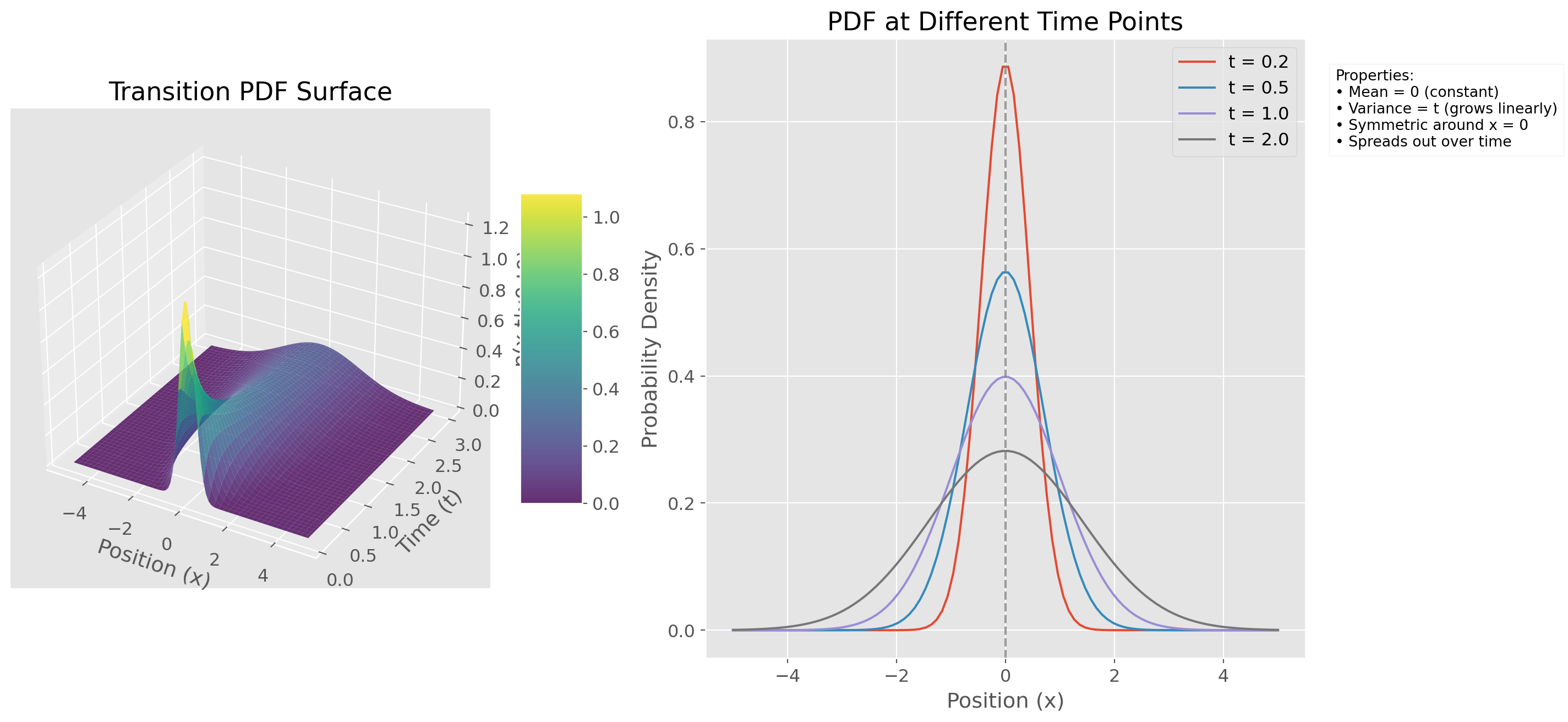
Fokker-Planck Equation
The Fokker-Planck Equation
The Fokker-Planck equation describes the time evolution of the probability density function for a stochastic process. It can be derived by applying the infinitesimal generator \(\mathcal{L}\) to the transition probability density:
\[ \frac{\partial p}{\partial t}=\mathcal{L} p=-\frac{\partial}{\partial x}[a(x, t) p]+\frac{1}{2} \frac{\partial^2}{\partial x^2}[\sigma^2(x, t) p] \]
Physical Interpretation
The equation has two main terms:
- Drift Term (\(-\frac{\partial}{\partial x}[a(x,t)p]\)):
- Represents deterministic motion
- \(a(x,t)\) is the drift coefficient
- Causes translation of the probability distribution
- Diffusion Term (\(\frac{1}{2}\frac{\partial^2}{\partial x^2}[\sigma^2(x,t)p]\)):
- Represents random fluctuations
- \(\sigma^2(x,t)\) is the diffusion coefficient
- Causes spreading of the probability distribution
Properties
- Conserves total probability: \(\int_{-\infty}^{\infty} p(x,t) dx = 1\) for all \(t\)
- For pure diffusion (\(a=0\), constant \(\sigma\)), solutions are Gaussian
- Time evolution preserves positivity: if \(p \geq 0\) initially, it remains so
- Special case of more general transport equations in physics
Brownian Motion in Fokker-Planck Equation
For Brownian motion, drift is \(0\), i.e. \(a(x, t) = 0\), diffusion is \(\sigma^2\). \[ \frac{\partial p(x, t)}{\partial t}=\frac{1}{2} \frac{\partial^2}{\partial x^2}\left[\sigma^2 p(x, t)\right] \]
Since \(\sigma\) is constant, we can take it outside the derivative: \[ \frac{\partial p(x, t)}{\partial t}=\frac{\sigma^2}{2} \frac{\partial^2 p(x, t)}{\partial x^2} \]
Numerical Solution of the Fokker-Planck Equation
The Fokker-Planck equation for Brownian motion is a partial differential equation (PDE) that describes the time evolution of the probability density function. For pure Brownian motion with diffusion coefficient \(\sigma\), it takes the form:
\[ \frac{\partial p}{\partial t} = \frac{\sigma^2}{2} \frac{\partial^2 p}{\partial x^2} \]
Numerical Method
We solve this equation using the finite difference method with the following components:
- Spatial Discretization:
- Domain: \([-L, L]\) divided into \(N_x\) points
- Central difference for second derivative: \[ \frac{\partial^2 p}{\partial x^2} \approx \frac{p_{i+1} - 2p_i + p_{i-1}}{\Delta x^2} \]
- Temporal Discretization:
- Forward Euler scheme: \[ \frac{p^{n+1}_i - p^n_i}{\Delta t} = \frac{\sigma^2}{2} \frac{p^n_{i+1} - 2p^n_i + p^n_{i-1}}{\Delta x^2} \]
- Boundary Conditions:
- Zero-flux boundary conditions at \(x = \pm L\)
- Implemented as \(p_0 = p_1\) and \(p_{N-1} = p_{N-2}\)
- Initial Condition:
- Narrow Gaussian distribution centered at \(x = 0\)
- Width chosen to be compatible with grid spacing
Numerical Stability
The numerical scheme is subject to the CFL (Courant-Friedrichs-Lewy) condition: \[ \frac{\sigma^2 \Delta t}{2\Delta x^2} \leq \frac{1}{2} \]
This condition ensures the numerical solution remains stable. The code checks this condition and warns if it might be violated.
Analysis and Validation
The numerical solution is validated by checking:
- Conservation of Probability: The total probability should remain 1
- Mean Position: Should remain at 0 due to symmetry
- Variance: Should grow linearly with time as \(\sigma^2 t\)
- Shape: Should maintain Gaussian form with increasing width
# Numerical Solution of the Fokker-Planck Equation for Brownian Motion
def solve_fokker_planck(sigma=1.0, L=10, Nx=100, Nt=100, T=1.0):
"""
Solve the Fokker-Planck equation for Brownian motion using finite differences.
Parameters:
-----------
sigma : float
Diffusion coefficient
L : float
Domain length (from -L to L)
Nx : int
Number of spatial points
Nt : int
Number of time points
T : float
Total simulation time
Returns:
--------
x : ndarray
Spatial grid points
t : ndarray
Time points
p : ndarray
Solution array (probability density function)
"""
# Derived parameters
D = sigma**2 / 2 # diffusion constant
x = np.linspace(-L, L, Nx) # spatial grid
t = np.linspace(0, T, Nt) # time grid
dx = x[1] - x[0]
dt = t[1] - t[0]
# Check numerical stability (CFL condition)
stability_param = D * dt / dx**2
if stability_param > 0.5:
print(f"Warning: Solution may be unstable! CFL number = {stability_param:.3f}")
# Initialize the probability density function
p = np.zeros((Nx, Nt))
# Initial condition: narrow Gaussian
initial_std = dx/2
p[:, 0] = stats.norm.pdf(x, loc=0, scale=initial_std)
# Time-stepping loop (Forward Euler scheme)
for n in range(0, Nt - 1):
# Interior points
for i in range(1, Nx - 1):
p[i, n + 1] = p[i, n] + D * dt / dx**2 * (
p[i + 1, n] - 2 * p[i, n] + p[i - 1, n]
)
# Boundary conditions (zero flux)
p[0, n + 1] = p[1, n + 1]
p[-1, n + 1] = p[-2, n + 1]
# Ensure conservation of probability
p[:, n+1] = p[:, n+1] / (np.sum(p[:, n+1]) * dx)
return x, t, p
def analyze_and_visualize_solution(x, t, p):
"""
Analyze and visualize the numerical solution.
"""
# Create figure with subplots
fig = plt.figure(figsize=(15, 10))
# 3D surface plot
ax1 = fig.add_subplot(221, projection='3d')
X, T = np.meshgrid(x, t)
surf = ax1.plot_surface(X, T, p.T, cmap='viridis')
ax1.set_xlabel('Position (x)')
ax1.set_ylabel('Time (t)')
ax1.set_zlabel('Probability Density')
ax1.set_title('Evolution of Probability Density')
fig.colorbar(surf, ax=ax1, shrink=0.5)
# Plot at selected times
ax2 = fig.add_subplot(222)
times = [0, int(len(t)/4), int(len(t)/2), -1]
for idx in times:
ax2.plot(x, p[:, idx], label=f't = {t[idx]:.2f}')
ax2.set_xlabel('Position (x)')
ax2.set_ylabel('Probability Density')
ax2.set_title('PDF at Different Times')
ax2.legend()
ax2.grid(True)
# Analyze statistical properties
ax3 = fig.add_subplot(223)
means = np.zeros(len(t))
variances = np.zeros(len(t))
for n in range(len(t)):
means[n] = np.sum(x * p[:, n]) * (x[1] - x[0])
variances[n] = np.sum((x - means[n])**2 * p[:, n]) * (x[1] - x[0])
ax3.plot(t, means, label='Mean')
ax3.plot(t, np.sqrt(variances), label='Standard Deviation')
ax3.set_xlabel('Time (t)')
ax3.set_ylabel('Value')
ax3.set_title('Evolution of Statistical Properties')
ax3.legend()
ax3.grid(True)
# Conservation check
ax4 = fig.add_subplot(224)
total_prob = np.sum(p, axis=0) * (x[1] - x[0])
ax4.plot(t, total_prob)
ax4.set_xlabel('Time (t)')
ax4.set_ylabel('Total Probability')
ax4.set_title('Conservation Check')
ax4.grid(True)
ax4.set_ylim([0.9, 1.1])
plt.tight_layout()
plt.show()
# Print analysis
print("\nNumerical Analysis:")
print(f"Final mean: {means[-1]:.6f} (should be close to 0)")
print(f"Final variance: {variances[-1]:.6f} (should be close to t = {t[-1]:.6f})")
print(f"Conservation error: {abs(1 - total_prob[-1]):.2e}")
# Solve the equation and visualize results
x, t, p = solve_fokker_planck(sigma=1.0, L=10, Nx=200, Nt=200, T=2.0)
analyze_and_visualize_solution(x, t, p)
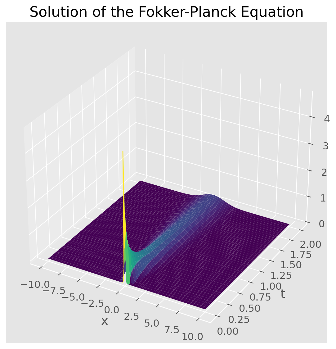
X, T = np.meshgrid(x, t)
fig = plt.figure(figsize=(10, 7))
ax = fig.add_subplot(111, projection="3d")
ax.plot_surface(X, T, p.T, cmap="viridis")
ax.set_xlabel("x")
ax.set_ylabel("t")
ax.set_zlabel("p(x, t)")
ax.set_title("Solution of the Fokker-Planck Equation")
plt.show()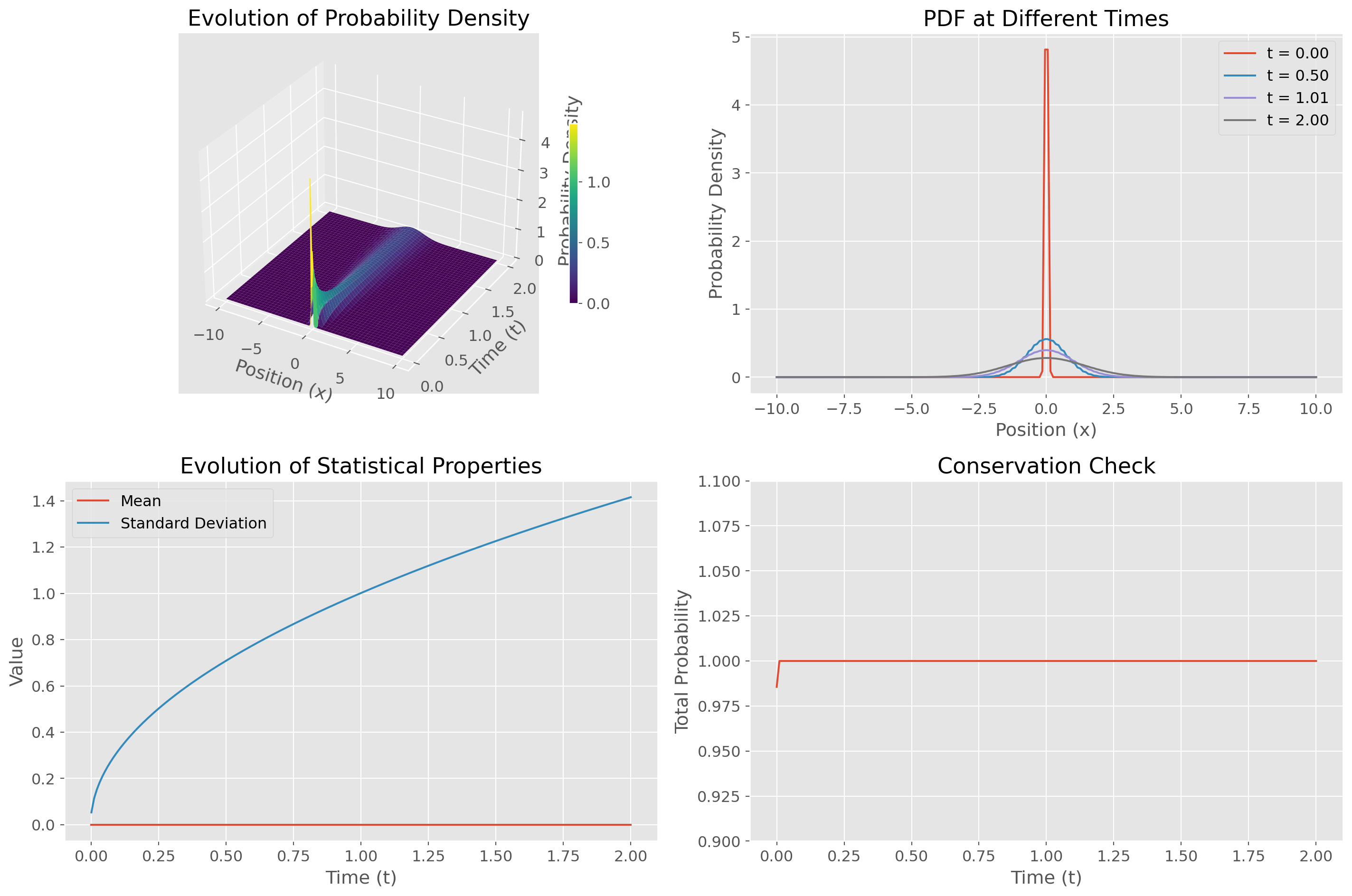
Numerical Analysis:
Final mean: 0.000000 (should be close to 0)
Final variance: 2.002889 (should be close to t = 2.000000)
Conservation error: 6.66e-16